PMSM Model

• IP core of a PMSM model

• Simulates a PMSM on the FPGA

• Intended for controller-in-the-loop (CIL) on the UltraZohm

• Time discrete transformation is done by zero order hold transformation

• Sample frequency of the integrator is \(T_s=\frac{1}{500\,kHz}\)

• IP core clock frequency must be \(f_{clk}=100\,MHz\)!

• IP core has single precision AXI ports

• All calculations in the IP core are done in single precision!

System description

Electrical System

The model assumes a symmetric machine with a sinusoidal input voltage as well as the common assumptions for the dq-transformation (neglecting the zero-component). Small letter values indicate time dependency without explicitly stating it.

Linear model

In the simplified linear case, the PMSM model is based on its differential equation using the flux-linkage as state values in the dq-plane [[2], p. 1092]:

\[ \begin{align}\begin{aligned}\frac{d \psi_d}{dt} &= u_d - R_1 i_d + \omega_{el} \psi_q\\\frac{d \psi_q}{dt} &= u_q - R_1 i_q - \omega_{el} \psi_d\end{aligned}\end{align} \]

The flux-linkages of the direct and quadrature axis are given by [[2], p. 1092]:

\[ \begin{align}\begin{aligned}\psi_d &= \psi_{pm} + L_d i_d\\\psi_q &= L_q i_q\end{aligned}\end{align} \]

Rearranging to calculate the current from the flux-linkage:

\[ \begin{align}\begin{aligned}i_d &= \frac{\psi_d - \psi_{pm}}{L_d}\\i_q &= \frac{\psi_q}{L_q}\end{aligned}\end{align} \]

With the rotational speed linked to the electrical rotation speed in dq-coordinates by the number of pole pairs [[2], p. 1092]:

\[\omega_{el}=p \cdot \omega_{mech}\]

The PMSM generates an inner torque \(T_I\) according to:

\[T_I=\frac{3}{2}p(\psi_d i_q - \psi_q i_d)\]

This can be rearranged to the following equation [[2], p. 1092]. Note that the flux-based equation above is implemented in the model.

\[T_I=\frac{3}{2} p \big(i_q \psi_{pm} + i_d i_q (L_d -L_q) \big)\]

Model with non-linear effects

This model takes saturation and cross-coupling effects into consideration. The flux-linkage is now dependent on the dq-currrents.

\[ \begin{align}\begin{aligned}\frac{d\psi_d}{dt} = \frac{\partial \psi_d}{\partial i_d}\frac{di_d}{dt}+ \frac{\partial \psi_d}{\partial i_q}\frac{di_q}{dt}\\\frac{d\psi_q}{dt} = \frac{\partial \psi_q}{\partial i_d}\frac{di_d}{dt}+ \frac{\partial \psi_q}{\partial i_q}\frac{di_q}{dt}\end{aligned}\end{align} \]

For the partial derivatives of the flux with respect to the currents, abbreviations are introduced. These are called differential self-inductances \(L_{dd}\) and \(L_{qq}\), as well as the differential cross-coupling inductances \(L_{dq}\) and \(L_{qd}\).

\[ \begin{align}\begin{aligned}L_{dd} = \frac{\partial \psi_{d}^{\left(i_{d},i_{q}\right)}}{\partial i_{d}}\\L_{qq} = \frac{\partial \psi_{q}^{\left(i_{d},i_{q}\right)}}{\partial i_{q}}\\L_{dq} = \frac{\partial \psi_{d}^{\left(i_{d},i_{q}\right)}}{\partial i_{q}}\\L_{qd} = \frac{\partial \psi_{q}^{\left(i_{d},i_{q}\right)}}{\partial i_{d}}\end{aligned}\end{align} \]

Rearranging the equations again to calculate the current from the flux-linkage:

\[ \begin{align}\begin{aligned}\frac{di_{d}}{dt}=\frac{u_{d}-R_{s}\cdot i_{d}-L_{dq} \frac{di_{q}}{dt}+\omega_{el} \psi_{q}}{L_{dd}}\\\frac{di_{q}}{dt}=\frac{u_{q}-R_{s} \cdot i_{q}-L_{qd} \frac{di_{d}}{dt}-\omega_{el} \psi_{d}}{L_{qq}}\end{aligned}\end{align} \]

The inner torque \(T_I\) is calculated using the flux-linkages.

\[T_I=\frac{3}{2}p(\psi_d(i_d,i_q) i_q - \psi_q(i_d,i_q) i_d)\]

Mechanical system

The mechanical system is modeled by the following equations. The inertia of the complete system is summed into the inertia \(J_{sum}\), i.e., rigid coupling of the system is assumed.

\[\frac{d \omega_{mech}}{dt} = \frac{ T_I - T_F - T_L }{J_{sum}}\]

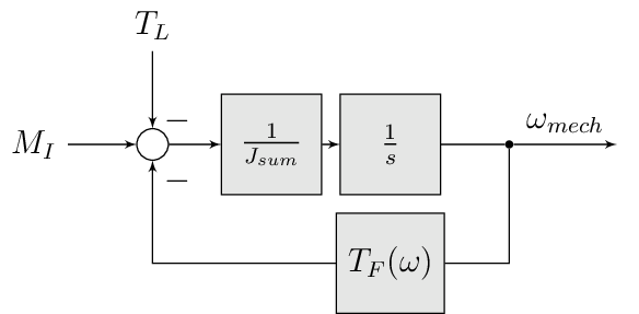
Fig. 360 Block diagram of mechanical system

Friction

The friction \(M_F(\omega)\) [ [1], p. 12 ff] is implemented with the simplified viscous friction model:

\[M_F = sign(\omega_{mech}) \cdot M_c + \sigma \omega_{mech}\]

With the constant coulomb friction \(M_c\), and the friction coefficient \(\sigma\).

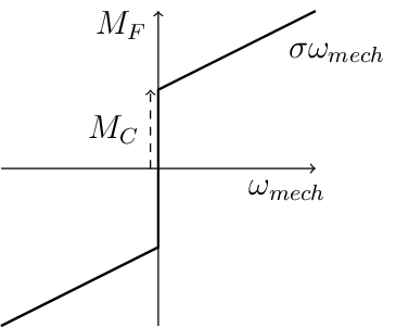
Fig. 361 Friction model [ [1], p. 13]

IP core overview

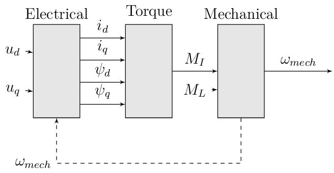
Fig. 362 Block diagram of IP core

All time-dependent variables are either inputs or outputs that are written/read by AXI4-full. That is, \(u_d\), \(u_q\), \(\omega_{mech}\), and \(M_L\) are inputs. Furthermore, \(i_d\), \(i_q\), \(M_I\), and \(\omega_{mech}\) are outputs. The IP core inputs \(\boldsymbol{u}(k)=[{v}_{d} ~ v_{q} ~ T_{L}]\) and outputs \(\boldsymbol{y}(k)=[i_{d} ~ i_{q} ~ T_{L} ~ \omega_{m}]\) are accessible by AXI4 (including burst transactions). Furthermore, all machine parameters, e.g., stator resistance, can be written by AXI at runtime. All AXI-transactions use single-precision variables. The inputs \(\boldsymbol{u}(k)\) and outputs \(\boldsymbol{y}(k)\) use a shadow register that holds the value of the register until a sample signal is triggered. Upon triggering, the inputs from the shadow register are passed to the actual input registers of the IP core, and the current output \(\boldsymbol{y}(k)\) is stored in the output shadow register (strobe functions of driver). The shadow registers can be triggered according to the requirements of the controller in the loop and ensure synchronous read/write operations. The inputs and outputs are implemented as an vector, therefore the HDL-Coder adds the strobe / shadow register automatically - it is not visible in the model itself. Note that \(\omega_{mech}\) is an input as well as an output. The IP core has two modes regarding the rotational speed \(\omega_{mech}\):

1. Simulate the mechanical system and calcualte \(\omega_{mech}\) according to the equations in Friction.

2. Use the rotational frequency \(\omega_{mech}\) that is written as an input (written by AXI).

When the flag simulate_mechanical_system is true, the rotational speed in the output struct is calculated by the IP core, and the input value of the rotational speed has no effect. When the flag simulate_mechanical_system is false, the rotational speed in the output struct is equal to the rotational speed of the input. This behavior is implemented in the hardware of the IP core with switches. The IP core also has a mode regarding saturation and cross-coupling effects. When the flag simulate_nonlinear is true, the flux-linkages \(\psi_d\) and \(\psi_q\) are dependent on the currents with the equations in Model with non-linear effects. When the flag simulate_nonlinear is false, the flux-linkages are used as state values with the equations in Linear model. The input and output values are intended to be written and read in a periodical function, e.g., the ISR.

In addition to the time-dependent values, the PMSM model parameters are configured by AXI.

Integration

The differential equations of the electrical and mechanical system are discretized using the explicit Euler method [ [3], p. 3 ]. Using this method is justified by the small integration step of the implementation (\(t_s=0.5~\mu s\)) and is a commonly used approach [3], p. 3 ]. The new value at time \(k+1\) of the state variable is calcualted for every time step based on the old values (\(k\)):

\[ \begin{align}\begin{aligned}\psi_d(k+1) &= t_s \bigg( u_d(k) - R_1 i_d(k) + \omega_{el} \psi_q(k) \bigg) + \psi_d(k)\\\psi_q(k+1) &=t_s \bigg( u_q(k) - R_1 i_q(k) - \omega_{el} \psi_d(k) \bigg) + \psi_q(k)\end{aligned}\end{align} \]

For the mechanical system:

\[\omega_{mech}(k+1) =ts \bigg( \frac{ T_I(k) - T_F(k) - T_L(k) }{J_{sum}} \bigg) + \omega_{mech}(k)\]

IP Core Hardware

• The module uses single precision.

• All input values are adjustable at run-time

• The sample time is fixed!

• The IP core uses Native Floating Point of the HDL-Coder

• Several parameters are written as their reciprocal to the AXI register to make the calculations on hardware simple (handled by the driver!)

• The IP core uses an oversampling factor of 200

• Floating Point latency Strategy is set to MIN

• Handle denormals is activated

Fig. 363 Test bench of PMSM plant model

Fig. 364 Overview of PMSM IP core

Fig. 365 Calculation of PMSM subsystem

Fig. 366 Torque calculation subsystem

Fig. 367 Mechanical calculation subsystem

Example usage

Vivado

• Add IP core to Vivado and connect to AXI (smartconnect)

• Source IPCORE_CLK with a \(100\,MHz\) clock!

• Connect other ports accordingly

• Assign address to IP core

• Build bitstream, export .xsa, update Vitis platform

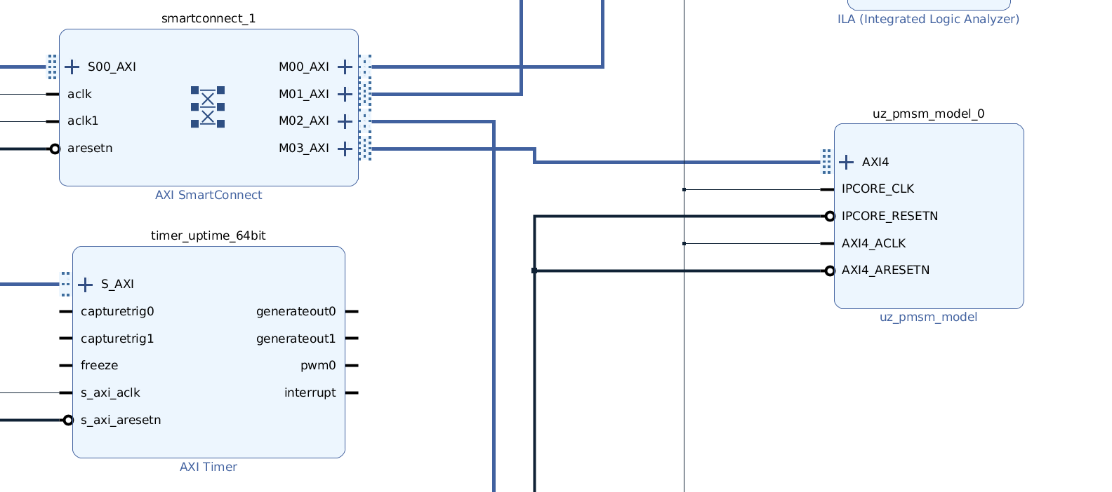
Fig. 368 Example connection of PMSM IP core

Vitis

• Initialize the driver in main and couple the base address with the driver instance

Listing 194 Changes in main.c (R5)

#include "IP_Cores/uz_pmsmMmodel/uz_pmsmModel.h"
#include "xparameters.h"
uz_pmsmModel_t *pmsm=NULL;

int main(void) {
// other code...

struct uz_pmsmModel_config_t pmsm_config={
  .base_address=XPAR_UZ_PMSM_MODEL_0_BASEADDR,
  .ip_core_frequency_Hz=100000000,
    .simulate_mechanical_system = true,
    .r_1 = 2.1f,
    .L_d = 0.03f,
    .L_q = 0.05f,
    .psi_pm = 0.05f,
    .polepairs = 2.0f,
    .inertia = 0.001,
    .coulomb_friction_constant = 0.01f,
    .friction_coefficient = 0.001f,
    .simulate_nonlinear = false;
    .ad1 = 0.0f,
                      .ad2 = 0.0f,
          .ad3 = 0.0f,
                      .ad4 = 0.0f,
                      .ad5 = 0.0f,
                      .ad6 = 0.0f,
                      .aq1 = 0.0f,
                      .aq2 = 0.0f,
                      .aq3 = 0.0f,
                      .aq4 = 0.0f,
                      .aq5 = 0.0f,
                      .aq6 = 0.0f,
                      .F1G1 = 0.0f,
                      .F2G2 = 0.0f};

pmsm=uz_pmsmModel_init(pmsm_config);
// before ISR Init!
// more code of main

• To determine the fitting parameters see Flux approximation script.

• Read and write the inputs in isr.c

• Add before ISR with global scope to use the driver and Waveform Generator:

Listing 195 Changes in isr.c

#include "../uz/uz_wavegen/uz_wavegen.h"
#include "../IP_Cores/uz_pmsmMmodel/uz_pmsmModel.h"
extern uz_pmsmModel_t *pmsm;

float i_d_soll=0.0f;
float i_q_soll=0.0f;
struct uz_pmsmModel_inputs_t pmsm_inputs={
    .omega_mech_1_s=0.0f,
    .v_d_V=0.0f,
    .v_q_V=0.0f,
    .load_torque=0.0f
};

struct uz_pmsmModel_outputs_t pmsm_outputs={
    .i_d_A=0.0f,
    .i_q_A=0.0f,
    .torque_Nm=0.0f,
    .omega_mech_1_s=0.0f
};

void ISR_Control(void *data){
// other code
uz_pmsmModel_trigger_input_strobe(pmsm);
      uz_pmsmModel_trigger_output_strobe(pmsm);
pmsm_outputs=uz_pmsmModel_get_outputs(pmsm);
pmsm_inputs.v_q_V=uz_wavegen_pulse(10.0f, 0.10f, 0.5f);
pmsm_inputs.v_d_V=-pmsm_inputs.v_q_V;
uz_pmsmModel_set_inputs(pmsm, pmsm_inputs);
// [...]
}

• Change the Javascope enum to transfer the required measurement data

Listing 196 Adjust JS_OberservableData enum in javascope.h (R5) to measure pmsm_outputs

// Do not change the first (zero) and last (end) entries.
enum JS_OberservableData {
  JSO_ZEROVALUE=0,
  JSO_i_q,
  JSO_i_d,
  JSO_omega,
  JSO_v_d,
  JSO_ENDMARKER
};

• Configure the Javascope to transmit the pmsm output data:

Listing 197 Adjust JavaScope_initalize function in javascope.c (R5) to measure pmsm_outputs

  #include "../IP_Cores/uz_pmsmMmodel/uz_pmsmModel.h"
  extern struct uz_pmsmModel_outputs_t pmsm_outputs;
  extern struct uz_pmsmModel_inputs_t pmsm_inputs;

  int JavaScope_initalize(DS_Data* data){
  // existing code
  // [...]
  // Store every observable signal into the Pointer-Array.
  // With the JavaScope, 4 signals can be displayed simultaneously
  // Changing between the observable signals is possible at runtime in the JavaScope.
  // the addresses in Global_Data do not change during runtime, this can be done in the init
  js_ch_observable[JSO_i_q] = &pmsm_outputs.i_q_A;
  js_ch_observable[JSO_i_d] = &pmsm_outputs.i_d_A;
  js_ch_observable[JSO_omega] = &pmsm_outputs.omega_mech_1_s;
  js_ch_observable[JSO_v_d] = &pmsm_inputs.v_d_V;
  return Status;
  }

Javascope

• Make sure that in properties.ini, smallestTimeStepUSEC = 50 is set

Flux approximation

The flux-linkages are approximated using analytic-Prototype functions. This is based on the approach and findings from [4]. For a more in depth look at the derivation, see [ [5], p. 30 ].

The entire range of the flux-linkages can be approximated with the following equations. Note that the terms \(\int \hat{\psi}_{cross}^{q,s1}(I_{q1}) di_{q}\) and \(\int \hat{\psi}_{cross}^{d,s1}(I_{d1}) di_{d}\) are constant values and will be used in the fitting parameters.

\[\hat{\psi}_{d}(i_{d},i_{q}) = \hat{\psi}_{d,self}(i_{d}) - \underbrace{\frac{1}{\int \hat{\psi}_{cross}^{q,s1}(i_{q}) \, di_{q}} \left( \hat{\psi}_{cross}^{d,s1}(i_{d},i_{q}=I_{q1}) \right) \left( \int \hat{\psi}_{cross}^{q,s1}(i_{q}) \, di_{q} \right)}_{=\hat{\psi}_{cross}^{d}(i_{d},i_{q})}\]

\[\hat{\psi}_{q}(i_{d},i_{q}) = \hat{\psi}_{q,self}(i_{q}) - \underbrace{\frac{1}{\int \hat{\psi}_{cross}^{d,s1}(i_{d}) \, di_{d}} \left( \hat{\psi}_{cross}^{q,s1}(i_{d}=I_{d1},i_{q}) \right) \left( \int \hat{\psi}_{cross}^{d,s1}(i_{d}) \, di_{d} \right)}_{=\hat{\psi}_{cross}^{q}(i_{d},i_{q})}\]

Approximation Example usage

In this example usage, flux-linkages of an example motor are getting approximated.

• There needs to be a Excel data sheet in the same directory as the PMSM IP core at ultrazohm_sw\ip_cores\uz_pmsm_model.

• The naming in the script has to be adjusted.

Listing 198 Example to get data out of a Excel data sheet.

...
FluxMapData = readtable('FluxMapData_Prototyp_1000rpm_');
...

• Afterwards the area where the Array is in the excel sheet has to be specified.

Listing 199 Example to specify array location and size.

...
% Currents
id = FluxMapData{1,1:20};
iq = FluxMapData{22:41,1};
%Psi_d
psi_d = FluxMapData{43:62,1:20}*(1e-3);
%Psi_q
psi_q = FluxMapData{108:127,1:20}*(1e-3);
...

• To run the approximation script, first the uz_pmsm_model_init_parameter.m file has to be ran.

• If the the script ran successfully the fitting parameters are in the MATLAB workspace and can be used in the IP core for nonlinear behavior or for different use in the sw-framework.

Comparison between reference and IP core

• Program UltraZohm with included PMSM IP core and software as described above

• Start Javascope

• Connect to javascope, set scope to running and time scale to 100x

• Start logging of data after a falling edge on the setpoint and stop at the next fallning edge

• Copy measured .csv data to ultrazohm_sw/ip-cores/uz_pmsm_model

• Rename it to open_loop_mearuement.csv

• Run compare_simulation_to_measurement.m in ultrazohm_sw/ip-cores/uz_pmsm_model

Fig. 369 Comparison of step response between the reference model and IP core implementation measured by Javascope

Closed loop

uz_pmsmModel_trigger_input_strobe(pmsm);
uz_pmsmModel_trigger_output_strobe(pmsm);
pmsm_outputs=uz_pmsmModel_get_outputs(pmsm);
referenceValue=uz_wavegen_pulse(1.0f, 0.10f, 0.5f);
pmsm_inputs.v_q_V=uz_PI_Controller_sample(pi_q, referenceValue, pmsm_outputs_old.i_q_A, false);
pmsm_inputs.v_d_V=uz_PI_Controller_sample(pi_d, -referenceValue, pmsm_outputs_old.i_d_A, false);
pmsm_inputs.v_q_V+=pmsm_config.polepairs*pmsm_outputs_old.omega_mech_1_s*(pmsm_config.L_d*pmsm_outputs_old.i_d_A+pmsm_config.psi_pm);
pmsm_inputs.v_d_V-=pmsm_config.polepairs*pmsm_outputs_old.omega_mech_1_s*(pmsm_config.L_q*pmsm_outputs_old.i_q_A);
uz_pmsmModel_set_inputs(pmsm, pmsm_inputs);
pmsm_outputs_old=pmsm_outputs;

Driver reference

typedef struct uz_pmsmModel_t uz_pmsmModel_t

Object data type definition of the PMSM model IP-Core driver.

struct uz_pmsmModel_config_t

Configuration struct for the PMSM model IP-Core driver.

Public Members

uint32_t base_address

Base address of the IP-Core instance to which the driver is coupled

uint32_t ip_core_frequency_Hz

Clock frequency of IP-Core

float polepairs

Pole pairs of the PMSM

float r_1

Stator resistance in ohm

float L_d

Direct inductance in Henry

float L_q

Quadrature inductance in Henry

float psi_pm

Linked magnetic flux of PM magnets

float friction_coefficient

Linear coefficient of friction

float coulomb_friction_constant

Static friction constant

float inertia

Inertia of the PMSM

bool simulate_mechanical_system

Determine if mechanical system is simulated or speed is an input

float ad1

Fitting Parameter for approximation of d- axis self saturation

float ad2

Fitting Parameter for approximation of d- axis self saturation

float ad3

Fitting Parameter for approximation of d- axis self saturation

float ad4

Fitting Parameter for approximation of d- axis cross-coupling saturation

float ad5

Fitting Parameter for approximation of d- axis cross-coupling saturation

float ad6

Fitting Parameter for approximation of d- axis cross-coupling saturation

float aq1

Fitting Parameter for approximation of q- axis self saturation

float aq2

Fitting Parameter for approximation of q- axis self saturation

float aq3

Fitting Parameter for approximation of q- axis self saturation

float aq4

Fitting Parameter for approximation of q- axis cross-coupling saturation

float aq5

Fitting Parameter for approximation of q- axis cross-coupling saturation

float aq6

Fitting Parameter for approximation of q- axis cross-coupling saturation

float F1G1

Fitting Parameter for cross-coupling approximation

float F2G2

Fitting Parameter for cross-coupling approximation

bool simulate_nonlinear

true: simulate nonlinear PMSM Model in the PL. Requires fitting parameters

struct uz_pmsmModel_outputs_t

Struct to return and read the outputs of the PMSM Model.

Public Members

float i_d_A

Current in d-axis in A

float i_q_A

Current in q-Axis in A

float torque_Nm

Inner torque of PMSM in Nm

float omega_mech_1_s

Rotational speed of PMSM in 1/s

struct uz_pmsmModel_inputs_t

Struct to be used to pass inputs to the PMSM Model.

Public Members

float v_d_V

Voltage in d-axis in V

float v_q_V

Voltage in q-axis in V

float omega_mech_1_s

Rotational speed of PMSM in 1/s

float load_torque

Applied load torque in Nm

uz_pmsmModel_t *uz_pmsmModel_init(struct uz_pmsmModel_config_t config)

Initialize an instance of the driver.

Parameters:

• config – Config struct

Returns:

uz_pmsmModel_t* Pointer to an initialized instance of the driver

void uz_pmsmModel_set_inputs(uz_pmsmModel_t *self, struct uz_pmsmModel_inputs_t inputs)

Takes the values of the shadow register and pass them to the actual AXI register.

Parameters:

• self –

struct uz_pmsmModel_outputs_t uz_pmsmModel_get_outputs(uz_pmsmModel_t *self)

Returns current outputs of PMSM model IP-Core.

Parameters:

• self – Pointer to driver instance

Returns:

struct uz_pmsmModel_outputs_t Output values

void uz_pmsmModel_reset(uz_pmsmModel_t *self)

Resets the PMSM model by writing zero to all inputs and sets integrators to zero.

Parameters:

• self – Pointer to driver instance

void uz_pmsmModel_trigger_input_strobe(uz_pmsmModel_t *self)

Takes the values of the AXI shadow register and pass them to the actual input.

Parameters:

• self –

void uz_pmsmModel_trigger_output_strobe(uz_pmsmModel_t *self)

Takes the values of the shadow register and pass them to the actual AXI register.

Parameters:

• self –

Sources

[1] (1,2)

Zur Modellierung und Kompensationdynamischer Reibung in Aktuatorsystemen, Michael Ruderman, Dissertation, 2012, TU Dortmund (German)

[2] (1,2,3,4)

Elektrische Antriebe - Regelung von Antriebssystemen, Dierk Schröder, Springer, 2015, 4. Edition (German)

[3] (1,2)

Exploring the Limits of Floating-Point Resolution for Hardware-In-the-Loop Implemented with FPGAs, Alberto Sanchez, Elías Todorovich, and Angel De Castro, Applications of Power Electronics, https://doi.org/10.3390/electronics7100219

[4]

Analytical Prototype Functions for Flux Linkage Approximation in Synchronous Machines, Shih-Wei Su, Christoph M. Hackl, and Ralph Kennel, IEEE Open Journal of the Industrial Electronics Society, vol. 3, pp. 265-282, 2022, doi: 10.1109/OJIES.2022.3162336

[5]

Feldorientierte Regelung von hoch ausgenutzten permanenterregten Synchronmaschinen, Philipp Dölger (German)