Space vector Modulation#
-
struct uz_DutyCycle_t#
Struct for the three DutyCycles for a three-phase-system.
-
struct uz_DutyCycle_2x3ph_t#
-
struct uz_DutyCycle_3x3ph_t#
-
struct uz_DutyCycle_t uz_Space_Vector_Modulation(uz_3ph_dq_t v_ref_Volts, float V_DC_Volts, float theta_el_rad)#
Generates a DutyCycle from dq-reference voltages via Space Vector Modulation for a carrier based PWM generation.
- Parameters:
v_ref_Volts – reference voltages in Volts (e.g. from current controller)
V_DC_Volts – DC-Link voltage in volts
theta_el_rad – electrical rotor angle in rad
- Returns:
struct uz_DutyCycle_t generated DutyCycles
Example#
1#include "uz/uz_Space_Vector_Modulation/uz_space_vector_modulation.h"
2int main(void) {
3   float V_DC_Volts = 24.0f;
4   float theta_el_rad = 100.0f;
5   uz_3ph_dq_t v_input_Volts = {.d = 5.0f, .q = 8.0f, .zero = 0.0f};
6   struct uz_DutyCycle_t output = uz_Space_Vector_Modulation(v_input_Volts, V_DC_Volts, theta_el_rad);
7}
Description#
Generates a DutyCycle from dq-reference voltages via Space Vector Limitation for a carrier based PWM generation. This is realized according to [[1]] . Further information can be found there.
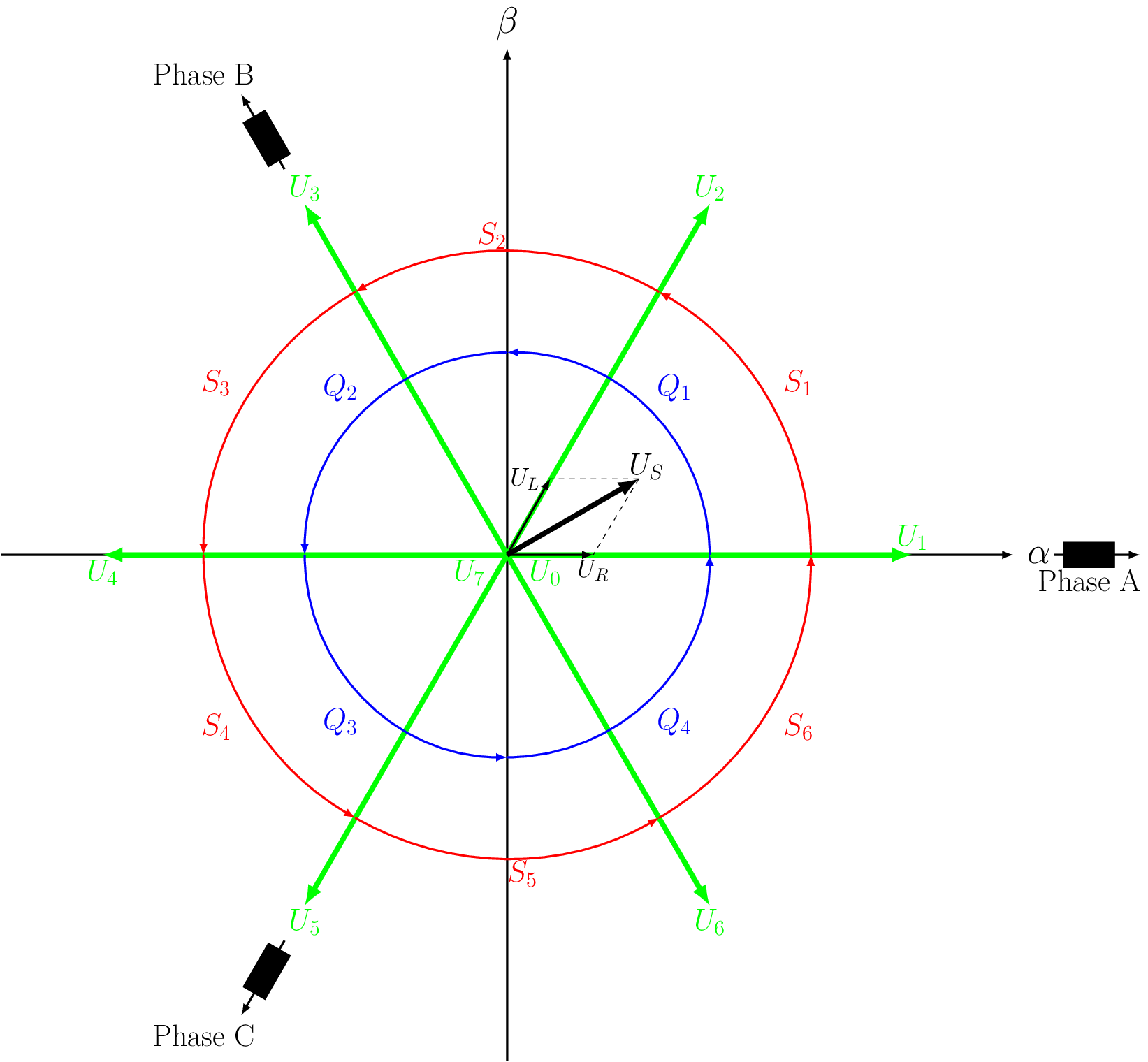
Fig. 392 Space vector coordinate system
Any arbitrary stator voltage vector can be produced from the eight standard vectors, which represent the eight possible logic states of a three phase voltage source inverter.
\(U_0\) |
\(U_1\) |
\(U_2\) |
\(U_3\) |
\(U_4\) |
\(U_5\) |
\(U_6\) |
\(U_7\) |
|
|---|---|---|---|---|---|---|---|---|
A |
0 |
1 |
1 |
0 |
0 |
0 |
1 |
1 |
B |
0 |
0 |
1 |
1 |
1 |
0 |
0 |
1 |
C |
0 |
0 |
0 |
0 |
1 |
1 |
1 |
1 |
\(U_S\) is achieved by vectorial addition of the two boundary vectors \(U_L\) and \(U_R\) in the directions of the standard vectors. This is achieved by modulating the on/off time of the two closest standard vectors and/or the two zero-voltage vectors (\(U_0, U_7\)). E.g. for the example provided in figure Fig. 392, a modulation between \(U_1, U_2\) and \(U_0\)/ \(U_7\) is required. Depending on the location of \(U_S\), the boundary vectors can be directly calculated from the \(\alpha\) and \(\beta\) voltages.
\(|U_R|\) |
\(|U_L|\) |
||
|---|---|---|---|
\(|S_1|\) |
\(|Q_1|\) |
\(|U_{\alpha}| - \frac{1}{\sqrt{3}}|U_{\beta}|\) |
\(\frac{2}{\sqrt{3}}|U_{\beta}|\) |
\(|S_2|\) |
\(|Q_1|\) |
\(|U_{\alpha}| + \frac{1}{\sqrt{3}}|U_{\beta}|\) |
\(-|U_{\alpha}| + \frac{1}{\sqrt{3}}|U_{\beta}|\) |
\(|S_2|\) |
\(|Q_2|\) |
\(-|U_{\alpha}| + \frac{1}{\sqrt{3}}|U_{\beta}|\) |
\(|U_{\alpha}| + \frac{1}{\sqrt{3}}|U_{\beta}|\) |
\(|S_3|\) |
\(|Q_2|\) |
\(\frac{2}{\sqrt{3}}|U_{\beta}|\) |
\(|U_{\alpha}| - \frac{1}{\sqrt{3}}|U_{\beta}|\) |
\(|S_4|\) |
\(|Q_3|\) |
\(|U_{\alpha}| - \frac{1}{\sqrt{3}}|U_{\beta}|\) |
\(\frac{2}{\sqrt{3}}|U_{\beta}|\) |
\(|S_5|\) |
\(|Q_3|\) |
\(|U_{\alpha}| + \frac{1}{\sqrt{3}}|U_{\beta}|\) |
\(-|U_{\alpha}| + \frac{1}{\sqrt{3}}|U_{\beta}|\) |
\(|S_5|\) |
\(|Q_4|\) |
\(-|U_{\alpha}| + \frac{1}{\sqrt{3}}|U_{\beta}|\) |
\(|U_{\alpha}| + \frac{1}{\sqrt{3}}|U_{\beta}|\) |
\(|S_6|\) |
\(|Q_4|\) |
\(\frac{2}{\sqrt{3}}|U_{\beta}|\) |
\(|U_{\alpha}| - \frac{1}{\sqrt{3}}|U_{\beta}|\) |
Depending on the current sector and quadrant, the appropriate boundary vectors \(U_L\) and \(U_R\) will be calculated and converted into DutyCycles. The DutyCycles are limited with the Saturation function to 1, respectively 0.